Bandit Algorithms

A better alternative to A/B testing

You’ve trained a model and it’s good. Maybe even great. It goes into production and everyone is happy.

After some time passes, you discover a new feature that will improve model performance. So you train a new model — one that includes this new feature. On the held out test data, everything looks good. The new feature does, indeed, improve performance.

However, you’ve been around long enough to know that better performance on the test set doesn’t necessarily mean better performance in production. In order to be sure that the new model is an improvement over your existing model, you need to test it in production.

A/B Testing

The simplest approach to this do some kind of A/B testing. You put both models into production and serve users predictions from one of the two models, based on some criterion (generally a random split). After some time has passed, you compare user behavior for users served predictions from the champion (production) model against those that were served predictions from the challenger model.

If the latter is better, you have some degree of confidence that the new model is in fact better than the older model. You can either do a full-scale replacement, or gradually replace the predictions for increasingly large subsets of users, comparing to the champion model results along the way.

This isn’t a bad approach. However, no matter which model is better, while the trial runs, you are seving at least some of the users using an inferior model. We’d like to say that we should size groups A and B in such way that the majority of users are getting the better model - but the whole point of running the trial is that we dont know which model is going to be better.

What we need is a solution that will adjust the size of our groups dynamically, based on which model is doing better. One approach to this is to use multi-armed bandit.

Bandits

A multi-armed bandit algorithm, as originally conceived, describes a way to handle the following situation: you walk into a casino and see a bank of slot machines (one-armed bandits). You have reason to believe that the payout for these machines is different. How can you maximize your winnings?

Intuitively, the solution should be: spend as much time as possible playing the machine with the greatest expected payout. So then how do we identify the machine with the greatest payout?

One solution would be to choose a number, say 1000, and play each machine machine 1000 times. Once we have run all of these trials, we can say with some degree of certainty which machine has the greatest expected payout.

Using this strategy however, if there are n machines, we are only playing the best one 1/nth of the time. If during our trials, we find a good machine, we have to stop playing it after 1000 plays, which may be suboptimal. On the other hand, addition, if it becomes clear early on that a given machine is particularly bad, using this strategy, we’d still have to keep playing it until we reached 1000 plays.

It would be better for our strategy to be able to adapt to the information we get about the expected payout of each machine as we get it. At the same time, we want to ensure that every machine is visited enough times that we are able to form some hypothesis about its expected payout.

The key aspects here are: 1. there are finite (generally small) number of options with 2. payouts determined by unknown random events and 3. we are free to switch between options at will.

Outside of the world of casino gambling, this kind of scenerio might arise when determining investment allocations: how much capital should we invest in predictable options (e.g. blue chip stocks) vs riskier assets which potentially have a higher upside? And as the latter investments begin paying out (or not), how shall we reallocate our portfolio?

The answer that bandit algorithms propose is can be summarized as: make a hypothesis, based on past experience, as to which is the best option. Choose the best option most of the time. The rest of the time, explore the other available options and update our understanding of their payouts. When we find another option that seems to be better than our current best, mark that option as best, and beginning using it.

In this way, we can be mostly certain that, after some initial experiments, we will be choosing the best option most of the time. In addition, the bigger the difference between the best option and other rest, the sooner we can expect to mark it as best and begin using it most of the time.

The simplest formulation of this strategy is the so called epsilon greedy algorithm.

Epsilon Greedy

Given a set of options O={o_1, … , o_n}, each that produce an outcome o, a reward function P such that P(o) is a real number representing the reward associated with outcome o, and epsilon > 0 (generally epsilon = 0.1 is a good starting point), we use the following algorithm:

1. Initialize a set of average observed rewards, R={r_1, …, r_n} for each option to 0

2. While True (or until some stopping criteria is met):

   1. Generate a random number between 0 and 1

      1. if that number > epsilon:

         1. choose the option corresponding to highest average reward (i.e. O[i] such that i = indexof(argmax(R)). In the case of a tie, choose the first option with the highest reward.

      2. else:

         1. choose an option, o_i, from O uniformly at random

   2. use P to evaluation o_i and update r_i

That’s it.

The advantage of this is 1. it’s very simple to implement and 2. compared to a random A/B split, once the algorithm discovers which option is the best, we will be serving users with the best model 100*(1-epsilon)% of the time.

Simple python implementation:

import numpy as np
from numpy.random import default_rng


class EpsilonGreedyBandit():
    def __init__(self, arms, epsilon=0.1, seed=512):
        # the set of models that bandit is choosing between
        self.arms = arms

        # probability that we will explore vs exploit
        self.epsilon = epsilon

        # the number of times we have used this model/arm
        self.n_visits = [0 for _ in range(len(arms))]

        # the average reward we have received from this model/arm
        self.rewards = [0 for _ in range(len(arms))]

        self.rng = default_rng(seed)

    def run_trial(self):
        if self.rng.random() < self.epsilon:
            # explore!
            arm = rng.integers(0, len(self.arms))
        else:
            # exploit!
            arm = np.argmax(self.rewards)

        this_model = self.arms[arm]
        this_reward = this_model.get_reward()

        # update the mean reward from this arm with 
        self.rewards[arm] = (
            self.n_visits[arm] * (self.rewards[arm]/(self.n_visits[arm]+1))
            + this_reward/(self.n_visits[arm]+1)
        )
        # update num visits for this arm
        self.n_visits[arm] += 1

        return this_reward

Using the above definition for my epsilon greedy bandit, I can run a simulation to see how the bandit performs with different values of epsilon.

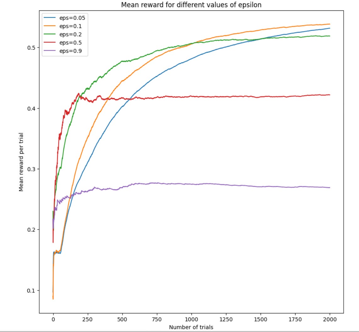
For this simulation, I presented the model with probabilities of success [0.1, 0.1, 0.3, 0.25, 0.6, 0.05] and ran 200 simulations for 2000 trials.

Two things here: first, it seems like the optimal value of epsilon is relatively small (<= roughly 0.2). This makes sense, as we want to exploit the best model we’ve found as much as possible, since it has the best chance of giving us a reward.

Second, the optimal amount that we should explore seems dependent on the number of trials that we run. If we are running < 500 trials, the best strategy seems to be exploring a bit more. Whereas if we are running a lot of trials 2000+, it seems like less exploration is better.

This roughly tracks with intuition, since the more trials we run, the more certainty we have about the underlying probabilties each of our arms give, so we don’t need to explore as much. We have increased certainity that our best choice is the best choice.

Epsilon Decreasing

With this in mind, we can consider a slight modification to the above: rather than sticking with a static epsilon, we can adjust epsilon downwards as we get more information. That is, we can start with a larger epsilon (lots of exploring), and as we get more information about the underlying distributions, we can shrink our epsilon and explore less.

This is generally done by introducing a new variable, alpha < 1. At each step, we decay epsilon by multiplying it by alpha. To ensure that we don’t decay epsilon away to 0, we can also introduce a lower boud to epsilon, which will ensure that we still do some exploring.

This updated bandit strategy is called Epsilon Decreasing.

class DecreasingBandit():
    def __init__(self, arms, epsilon, alpha, lower_bound, seed=512):
        self.arms = arms
        # the number of times we have used this model/arm
        self.n_visits = [0 for _ in range(len(arms))]
        # the average reward we have received from this model/arm
        self.rewards = [0 for _ in range(len(arms))]
        self.epsilon = epsilon
        self.alpha = alpha
        self.lower_bound = lower_bound

        self.rng = default_rng(seed)

    def run_trial(self):
        r = self.rng.random()

        if r < self.epsilon:
            arm = rng.integers(0, len(self.arms))
        else:
            arm = np.argmax(self.rewards)

        this_model = self.arms[arm]
        this_reward = this_model.get_reward()

        # update the mean reward from this arm with 
        self.rewards[arm] = (
            self.n_visits[arm] * (self.rewards[arm]/(self.n_visits[arm]+1))
            + this_reward/(self.n_visits[arm]+1)
        )
        # update num visits for this arm
        self.n_visits[arm] += 1

        # update epsilon
        self.epsilon = max(self.epsilon*self.alpha, self.lower_bound)
        
        return this_reward

Using a value of .999 for alpha (.1% decay) and 0.05 as the lower bound, we get the following rewards plot:

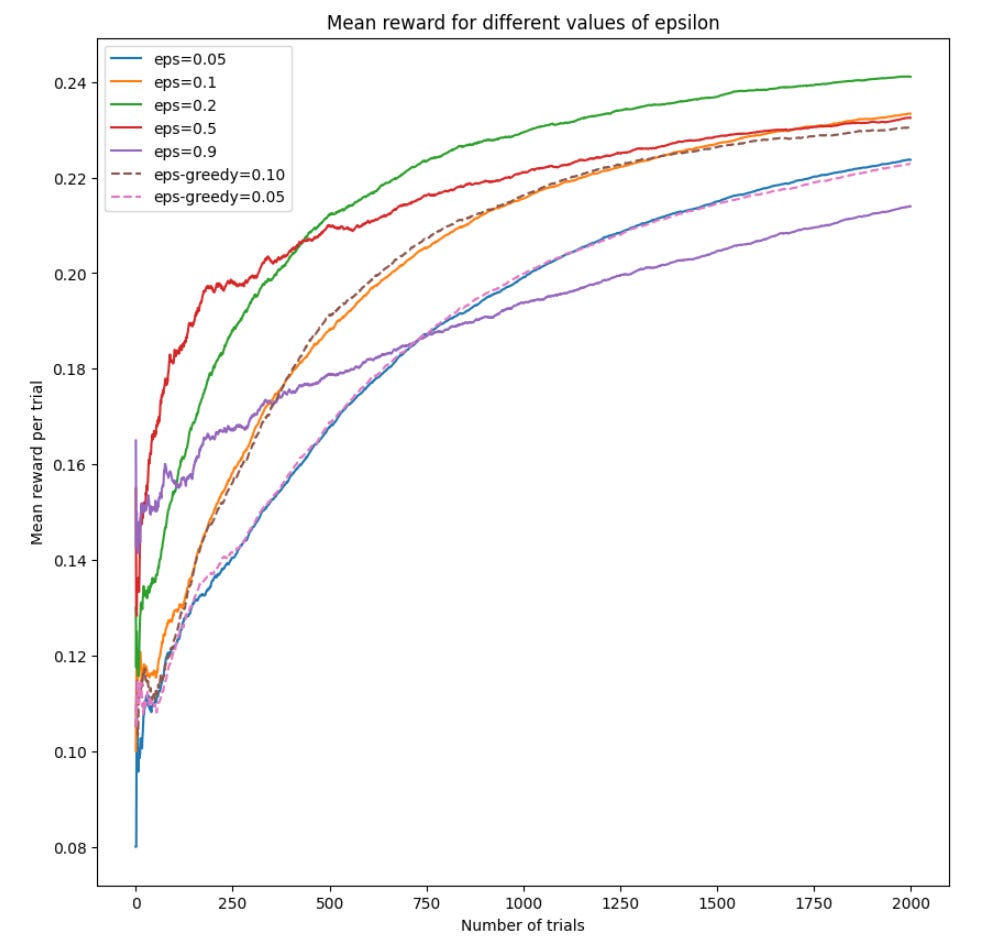
We see that this strategy out performs epsilon greedy. We also see that (not surprisingly), it favors higher exploration, since this will allow the model to find the true distributions more quickly without getting stuck endlessly exploring.

Other bandit algorithms

These are the simplest bandit algorithms, and as such, they are probably the ones that you should use most of the time. There is great value in simplicity and as long as the rewards for the more complicated algos aren’t spectacularly better (they’re not), you might as well do the simple thing that is unlikely to have implementation errors, etc.

However, we will mention that there are many other bandit algorithms including Upper Confidence Bound (UCB1) and Thompson sampling. These other algorithms are similar in that they deal with making the decision about when to explore and when to stay point (exploit).

The main difference between these algorithms and epsion greedy is the way the explorations are handled. Essentially, at the exploration stage, rather than just choosing randomly between all available arms, it might make sense to use the information we have gathered so far. For example, we might wish to select options for which there is a lot of uncertainty about their underlying distributions or possibly the option with the highest likelihood of paying out. At the same time, we should be avoiding options that we are confident have a lot payout.

Final words on bandit algorithms

Bandit algorithms are great for the situation I outlined above: we are testing one or several models in production, and we want to start using the best model as soon as possible.

However, this isn’t always the case. Models seldom exist in a void. There are often other considerations at play (cost of serving, user pivacy, cost of data, complexity of model, etc). In these cases, we might be using performance in production as one variable among many when deciding which model to choose.

In these cases, using an A/B test might be preferable, as it gives a clear measurement of the difference in performance among models plus a confidence interval. This information can be combined with other business considerations to arrive at a final decision about which model to use.