
Absolute Embeddings, Relative Embeddings
Some experiments with absolute embeddings; some experiments with relative positional embeddings


After my last post on absolute positional embeddings, I decided to run a few experiments to see how different static embedding schemas worked in practice.
For these experiments, I used Karpathy’s minGPT as my base transformer model and edited the positional encodings. I kept the training parameters and model architecture constant for each experiment, changing only the positional embedding scheme.
It is probably also worth noting that, due to lack of computing resources and budget, these experiments were done on a small (4 layers - 4 heads - 128 dimensions) character-level transformer (i.e., our tokens are characters, rather than words/word-pieces).
To begin, Karpathy uses absolute positional embeddings of dimension model_dim, which are learned along with the rest of the model weights. This is implemented as follows:
In the model’s __init__() function we have, which initializes the positional embeddings (wpe) using pytorch’s nn.Embedding() function. This essentially creates a matrix whose ith row is retrieved when the embedding object is passed i as an input. The optimal values for each of these rows are learned as the model is trained.
class GPT(nn.Module):

    def __init__(self, config):
        super().__init__()
        assert config.vocab_size is not None
        assert config.block_size is not None  # block size is max sequnece length
        self.config = config

        self.transformer = nn.ModuleDict(dict(
            wte = nn.Embedding(config.vocab_size, config.n_embd),
            wpe = nn.Embedding(config.block_size, config.n_embd),
            drop = nn.Dropout(config.dropout),
            h = nn.ModuleList([Block(config) for _ in range(config.n_layer)]),
            ln_f = LayerNorm(config.n_embd, bias=config.bias),
        ))
And then later, in the forward pass we have:
def forward(self, idx, targets=None):
        device = idx.device
        b, t = idx.size()
        assert t <= self.config.block_size, f"Cannot forward sequence of length {t}, block size is only {self.config.block_size}"
        pos = torch.arange(0, t, dtype=torch.long, device=device) # shape (t)

        # forward the GPT model itself
        tok_emb = self.transformer.wte(idx) # token embeddings of shape (b, t, n_embd)
        pos_emb = self.transformer.wpe(pos) # position embeddings of shape (t, n_embd)
        x = self.transformer.drop(tok_emb + pos_emb)
which retrieves the positional embeddings and adds them to the token embeddings before passing the sum to the transformer model.
Apart from the positional encoding scheme, this aligns with what we saw in Attention Is All You Need (AIAYN), which added the positional embeddings to the token embeddings and then passes the sum to the first transformer block.
As a baseline, we run the model without modification. This achieved around 1.64 as a minimum loss on the validation set.

As a first experiment, I disabled the positional encoding all together. This can be done simply by changing x = self.transformer.drop(tok_emb + pos_emb) to x = self.transformer.drop(tok_emb) in the forward step above.
Without the positional embeddings, the model is only able to achieve a minimum validation loss of around 1.76.
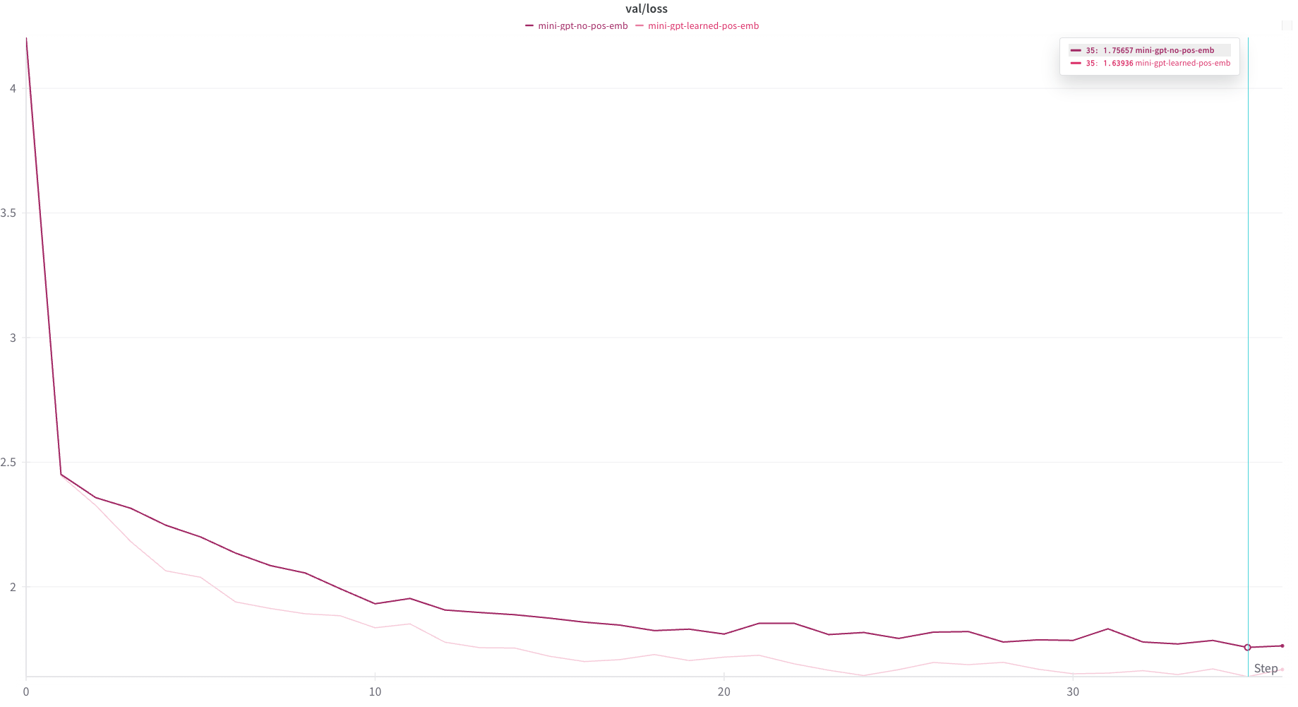
This gives some evidence that the positional encodings are doing something, which aligns with our expectations. However, it should also be noted that the model does pretty well just by treating the input as a “bag of letters”.
Next, I swapped out the learned positional embeddings with the static sinusoidal encodings described in AIAYN.
def get_positional_embedding(token_position, model_dim, const=10000):
"""
see: attention is all you need paper
"""
trig_ipt = lambda x: token_position/(const**(2*x/model_dim))
even_positions = np.sin(trig_ipt(np.arange(model_dim//2)))
odd_positions = np.cos(trig_ipt(np.arange(model_dim//2)))
output = np.zeros(model_dim)
output[0::2] = even_positions
output[1::2] = odd_positions
return output
### Further experiments will edit only this function
def get_pos_emb(config):
emb = nn.Embedding(config.block_size, config.n_embd)
new_emb = torch.tensor(
[get_positional_embedding(i, config.n_embd) for i in range(config.block_size)],
dtype=torch.float
)
emb.weight.data = new_emb
# freezing weights
emb.weight.requires_grad = False
return emb
### This is shown to illustrate where the function is being used
class GPT(nn.Module):
def __init__(self, config):
super().__init__()
assert config.vocab_size is not None
assert config.block_size is not None # block size is max sequnece length
self.config = config
self.transformer = nn.ModuleDict(dict(
wte = nn.Embedding(config.vocab_size, config.n_embd),
wpe = get_pos_emb(config),
drop = nn.Dropout(config.dropout),
h = nn.ModuleList([Block(config) for _ in range(config.n_layer)]),
ln_f = LayerNorm(config.n_embd, bias=config.bias),
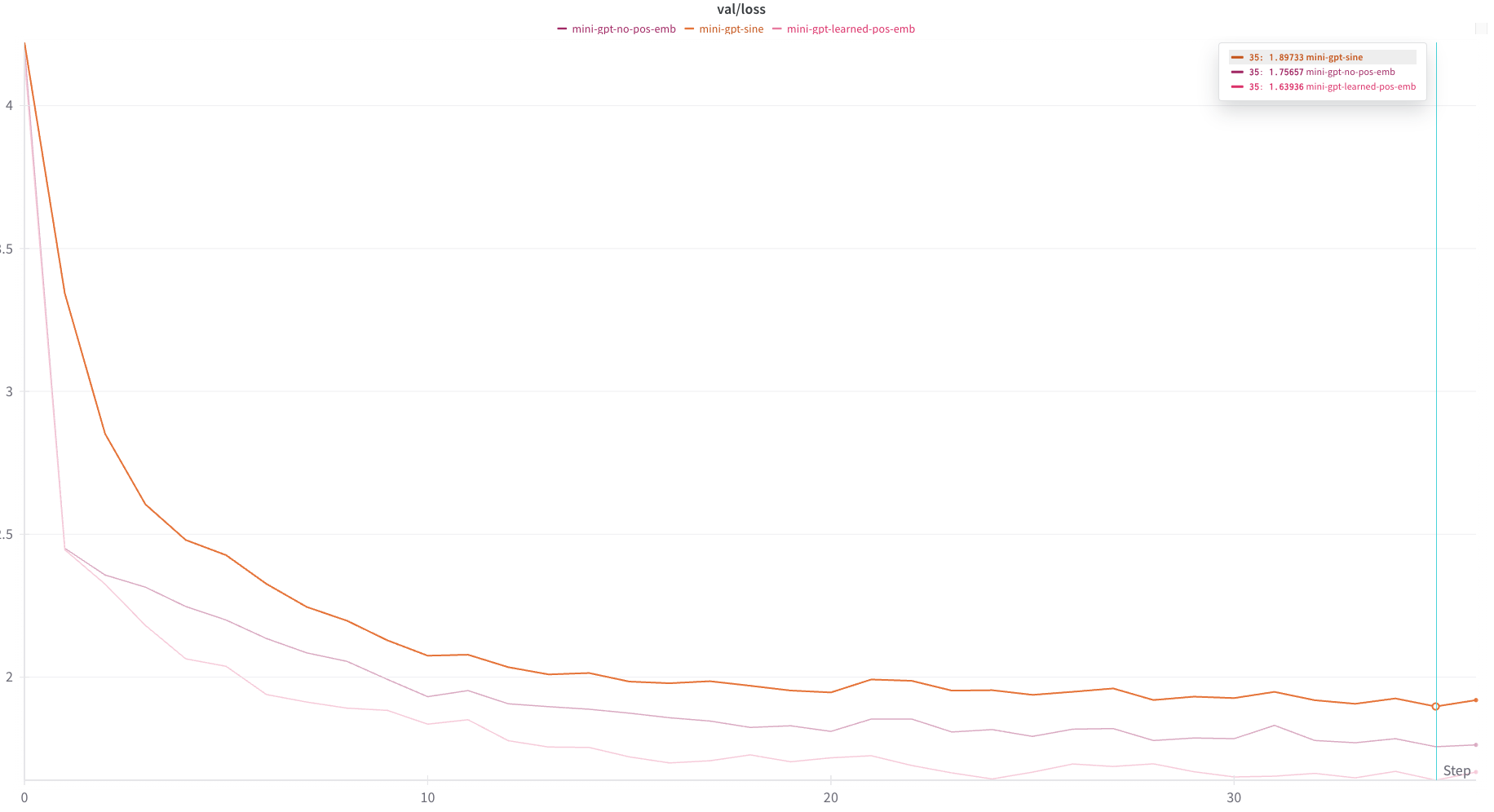
))Surprisingly, this schema performed much worse than having no embedding schema at all. My suspicion is that either 1. the trigonometric encoding was too complicated for the model to learn and extract the actual tokens from or 2. I have made an implementation error.
In any case, using the encoding scheme above, we achieve no better than about 1.9 validation loss:
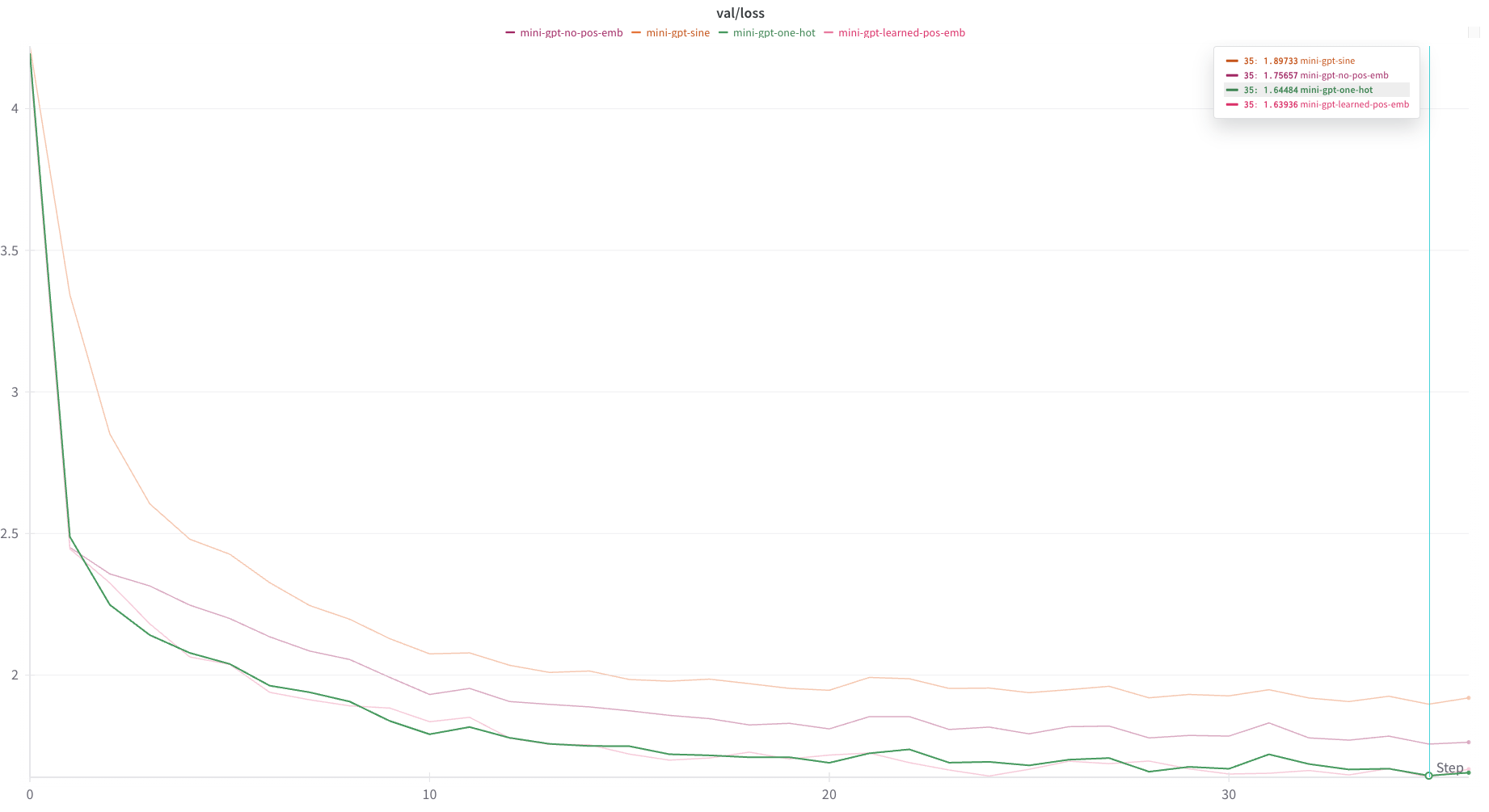
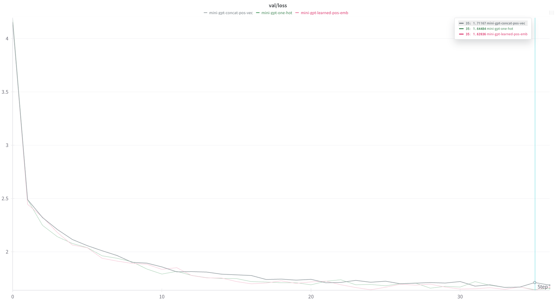
In an effort to present the model with the simplest position encoding that I could think of, my next experiments used a one-hot encoding scheme. Essentially, the ith token would receive a positional embedding whose jth entry is defined by the following function:
def get_pos_emb(config):
    emb = nn.Embedding(config.block_size, config.n_embd)

    new_emb = torch.zeros(config.block_size, config.n_embd)
    for i in range(config.block_size):
        new_emb[i][i] = 1.

    emb.weight.data = new_emb

    # freezing weights
    emb.weight.requires_grad = False

    return emb
This encoding schema achieved similar results to the learned encodings, indicating that the model is able to learn this encoding schema with about the same amount of effort that it uses to derive its own embedding schema.
As we shall see later, better results can be achieved with other positional encoding schemas. This perhaps indicates that the positional embeddings learned by the model (at least in this case) are may be as naive as those produced by the one-hot method.
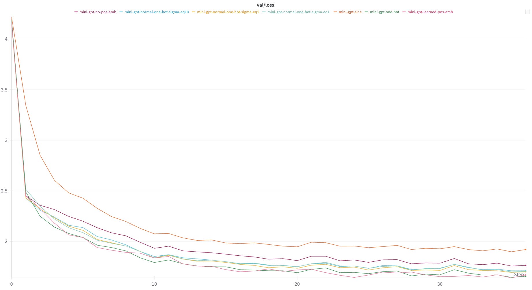
Feeling that this encoding schema might be too “peaky”, and that the model might do better with a smoother embedding, I experimented with smoothing the one_hot embedding by populating the positional encoding vectors with values drawn from a normal distribution centered at each position.
def get_pos_emb(config):
    emb = nn.Embedding(config.block_size, config.n_embd)

    sigma = 10
    new_emb = [
        stats.norm.pdf(
            np.linspace(max(0, i-3*sigma), i + 3*sigma, config.n_embd),
            i, sigma
            ) for i in range(config.block_size)
        ]
    new_emb = torch.tensor(new_emb, dtype=torch.float)

    emb.weight.data = new_emb

    # freezing weights
    emb.weight.requires_grad = False

    return emb
Results were worse than using the binary one-hot encoding (though better than using no encoding at all). Interestingly, the value of sigma did not seem to have much of an effect model performance — perhaps that all values of sigma I tried confused the model about the same amount.
The final experiment I ran was to get rid of the positional encodings altogether and instead add the token positions to the end of the token vector. I devoted 10 bits to this effort, which worked with input sequences up to a maximum length 1024, but reduced the token embedding dimension by 10.
## pos_emb definition
new_emb = [
   [int(i) for i in bin(num)[2:].zfill(10)]
   for i in range(config.block_size)
   ]
new_emb = torch.tensor(new_emb, dtype=torch.float)

## in the forward pass
tok_emb = self.transformer.wte(idx) # token embeddings of shape (b, t, n_embd)
pos_emb = self.transformer.wpe(pos) # position embeddings of shape (t, n_embd)

B,T,N = tok_emb.shape
ipt = torch.cat([tok_emb, pos_emb.expand(B, T, 10)], axis=2)

x = self.transformer.drop(ipt)
It’s also worth noting that minGPT uses weight_tying, which had to be disabled to get this to work.
Results were on par/marginally worse than learned embeddings and one-hot positional encodings.
Static absolute positional embeddings
While far from conclusive, I was not able to manually derive a positional encoding schema that outperformed learned positional embeddings. In most cases, my attempts produced worse results.
This should not be too surprising. Consider, the task is ultimately to derive a matrix P, that contains the encodings for every input position. Generally speaking, the best way to solve as task like this — especially when we have an easily articulated and differentiable loss function — is to learn the values of P using gradient descent. This is exactly what the learned embeddings schema do.
It should not be surprising that learning the best values of P using model training produces superior results to guessing them using intuition.
On the other hand, it is somewhat surprising that I was able to produce static embeddings that achieved results on-par with the learned positional embeddings. My takeaway here is that the embeddings being learned by the model are some combination of fairly simple and not super important to overall performance.
In any case, the small scale of this model and the problem on which it was trained make it hard to draw many definitive conclusions.
Relative positional embeddings
Soon after AIAYN was released, Shaw et al. released a paper describing a positional embedding scheme that replaces the absolute position embeddings with positional embeddings tokens’ relative positions.
The important observation here is that it’s not so important that token A falls at position i and token B falls at position j. What really matters is how i and j relate to each other. That is, does token B immediately follow token A? If so, then it probably has a lot of impact on the meaning of token A. On the other hand, if it occurs 100 tokens later, it probably has little bearing on A.
The other important change the authors propose is moving the positional embeddings into attention calculation, rather than adding them to the input vector. Thus allowing positional information to propagate deeper into the model.
Algorithm Description
To begin, the authors view the input tokens in terms of a directed, fully-connected graph. In this framing, we can create a vector a_{i,j}, which describes the edge connecting token i to token j. If we define a_{i,j} to have the same dimension as the token embeddings, we can then incorporate them in the attention layers.
The authors propose deriving two sets of these vectors, a_K and a_V, and updating the attention calculation as follows: First, a_K is added to key-query calculation (presumably to weight the key vectors by their relative proximity to the queries):
where W^Q and Q^K are the query and key matrices, respectively and d_z is the dimension of the token embeddings.
Recall that these e_i,j are then passed through a softmax function to produce a vector of \alpha_{i,j}’s. These \alpha_{i,j}’s are used to weight the value that we put on x_jW^V when calculating z_i, the output of the attention head at position i. The second set of vectors, a_V is added during this calculation:
It is worth noting here that the authors point out that this step may not be necessary, and found no difference in performance between models that included both a_K and a_V and models that only included a_K (they found models that only included a_V to perform worse than models with only a_K, but better than models without any position encoding). In fact, later work (e.g. this refinement by Huang et al.), they remove this step entirely.
Finally, a_V and a_K are shared between all the attention heads at each layer and every layer of the model learns its own a_V and a_K vectors.
After defining their position embedding schema, the authors of this paper hypothesize that relative token positions are only important up to a point. That is, they suggest that there may not be much difference between the relationship of a token to its 100th successor vs its 116th successor. Another way of stating this is that the only relative positions that matter are those that are “near” the token in question.
With this in mind, they suggest clipping token distance to a maximum of k. Tokens further than k positions from the input position will all be given the same position vector (technically one of two position vectors, depending on whether the token precedes or follows the target position).
The important thing is, rather than learning relationship vectors for every possible distance between two tokens (or, in the case where we limit the input sequence length to L, 2L+1 relationship vectors), we only need to learn 2k+1 (k tokens before the input position, the input position itself, and k tokens after the input position). The authors refer to this limited set of position embeddings as
To make this even more explicit, consider the following sentence:
I like to eat ice cream.
If we take k=3, this means that during the attention calculations for the first position (input token = "I”), we need use the following positional embedding vectors:
“I” gets positional embedding vectors w_0, since it is 0 positions away from the target position
“like” gets the positional embedding vectors w_1, since it is 1 position away
“to” gets the positional embedding vectors w_2 , since it is 2 positions away
“eat” gets the positional embedding vectors w_3, since it is 3 positions away
“ice” gets the positional embedding vectors w_3, because it is greater than 3 positions away, and we have capped our positional embeddings at 3
“cream” also gets positional embedding vectors w_3 for the reason stated above
That is, the set of positional embedding vectors used when calculating the attention head output for the first token are:
Similarly, the set of w_i used for the next two tokens are:
And the set of w_i used for the final token are:
I implemented this in pytorch using the following code.
First, because this positional embedding schema alters the attention head calculation, I created a new class, SelfAttentionWithRelativePOSEncoding, and initialized the two relative embedding matrices, rK and rV:
def __init__(self, config):
        super().__init__()
        assert config.n_embd % config.n_head == 0
        # key, query, value projections for all heads, but in a batch
        self.c_attn = nn.Linear(config.n_embd, 3 * config.n_embd, bias=config.bias)
        # output projection
        self.c_proj = nn.Linear(config.n_embd, config.n_embd, bias=config.bias)
        # postion_encodings
        self.rK = nn.Parameter(torch.rand(2*config.pos_k + 1, config.n_embd))
        self.rV = nn.Parameter(torch.rand(2*config.pos_k + 1, config.n_embd))
        # regularization
        self.attn_dropout = nn.Dropout(config.dropout)
        self.resid_dropout = nn.Dropout(config.dropout)
        self.n_head = config.n_head
        self.n_embd = config.n_embd
        self.dropout = config.dropout
        self.pos_k = config.pos_k
[Note: the current version of minGPT uses flash attention, which is implemented by a single pytorch call: torch.nn.functional.scaled_dot_product_attention(). Rather than trying to mess around with the pytorch internals, I chose to disable flash attention and use the manual attention calculation in the minGPT code base instead.]
We then need to add the positional embeddings to the attention calculations in the forward pass:
def forward(self, x):
        B, T, C = x.size() # batch size, sequence length, embedding dimensionality (n_embd)

        # calculate query, key, values for all heads in batch and move head forward to be the batch dim
        q, k, v  = self.c_attn(x).split(self.n_embd, dim=2)
        k = k.view(B, T, self.n_head, C // self.n_head).transpose(1, 2) # (B, nh, T, hs)
        q = q.view(B, T, self.n_head, C // self.n_head).transpose(1, 2) # (B, nh, T, hs)
        v = v.view(B, T, self.n_head, C // self.n_head).transpose(1, 2) # (B, nh, T, hs)

        # causal self-attention; Self-attend: (B, nh, T, hs) x (B, nh, hs, T) -> (B, nh, T, T)

        # manual implementation of attention
        att = (q @ k.transpose(-2, -1)) * (1.0 / math.sqrt(k.size(-1))) # B, nh, T, T
        # implementing eqn(1)
        att += self.multiply_by_rK(k) * (1.0 / math.sqrt(k.size(-1)))
        att = att.masked_fill(self.bias[:,:,:T,:T] == 0, float('-inf'))
        att = F.softmax(att, dim=-1)
        att = self.attn_dropout(att)
        y = att @ v  # (B, nh, T, T) x (B, nh, T, hs) + (B, nh, T, hs) -> (B, nh, T, hs)
        # implementing eqn(2)
        y += self.multiply_by_rV(att)

        y = y.transpose(1, 2).contiguous().view(B, T, C) # re-assemble all head outputs side by side

        # output projection
        y = self.resid_dropout(self.c_proj(y))
        return y
Where multiply_by_rK() and multiply_by_rV() are defined as:
def multiply_by_rK(self, k):
        B, nh, T, d_over_nh = k.shape  # batch_size, n_heads, sequence_length, model_dim/n_heads
        _k, d = self.rK.shape # 2*k+1, model_dim
        device = k.device

        rK = (
            self.rK.expand(B, _k, d)
            .view(B, _k, self.n_head, d_over_nh)
            .transpose(1,2)  # (B, hn, _k, d_over_nh)
        )

        pad = max(0, T-(self.pos_k+1))
        with torch.enable_grad():
            rK_padded = torch.nn.functional.pad(
                rK, (0, 0, pad, pad), mode='replicate'
                )

        pad = T - 2*self.pos_k - 1

        indices = torch.arange(T).unsqueeze(0) + torch.arange(T).unsqueeze(1)
        indices = indices.expand(B, self.n_head, T, T).to(device)

        res = (k.flip(2)@rK_padded.transpose(2, 3))   # we flip rows so we multiply tokens in reverse order
        res = res.gather(3, indices)
        return res.flip(2)  # restore original token order | shape = B, nh, T, T


def multiply_by_rV(self, attn):
        B, nh, T, T = attn.shape
        _k, d = self.rV.shape

        rV = (
            self.rV.expand(B, _k, d)
            .view(B, _k, self.n_head, d // nh)
            .transpose(1,2)  # (B, _k, T, d_over_nh)
        )

        pad = max(0, T-(self.pos_k+1))
        with torch.enable_grad():
            rV_padded = torch.nn.functional.pad(
                rV, (0, 0, pad, pad), mode='replicate'
                )

        indices = torch.arange(T).unsqueeze(0) + torch.arange(T).unsqueeze(1)

        # TODO: optimize this
        c = [attn.flip(2)[:, :, i:i+1, :]@rV_padded[:, :, ind, :] for i, ind in enumerate(indices)]
        return torch.concat(c, 2).flip(2)  # restore original token order | shape = B, nh, T, d_over_nh
Using this code and a value of k=4, I got the following results:
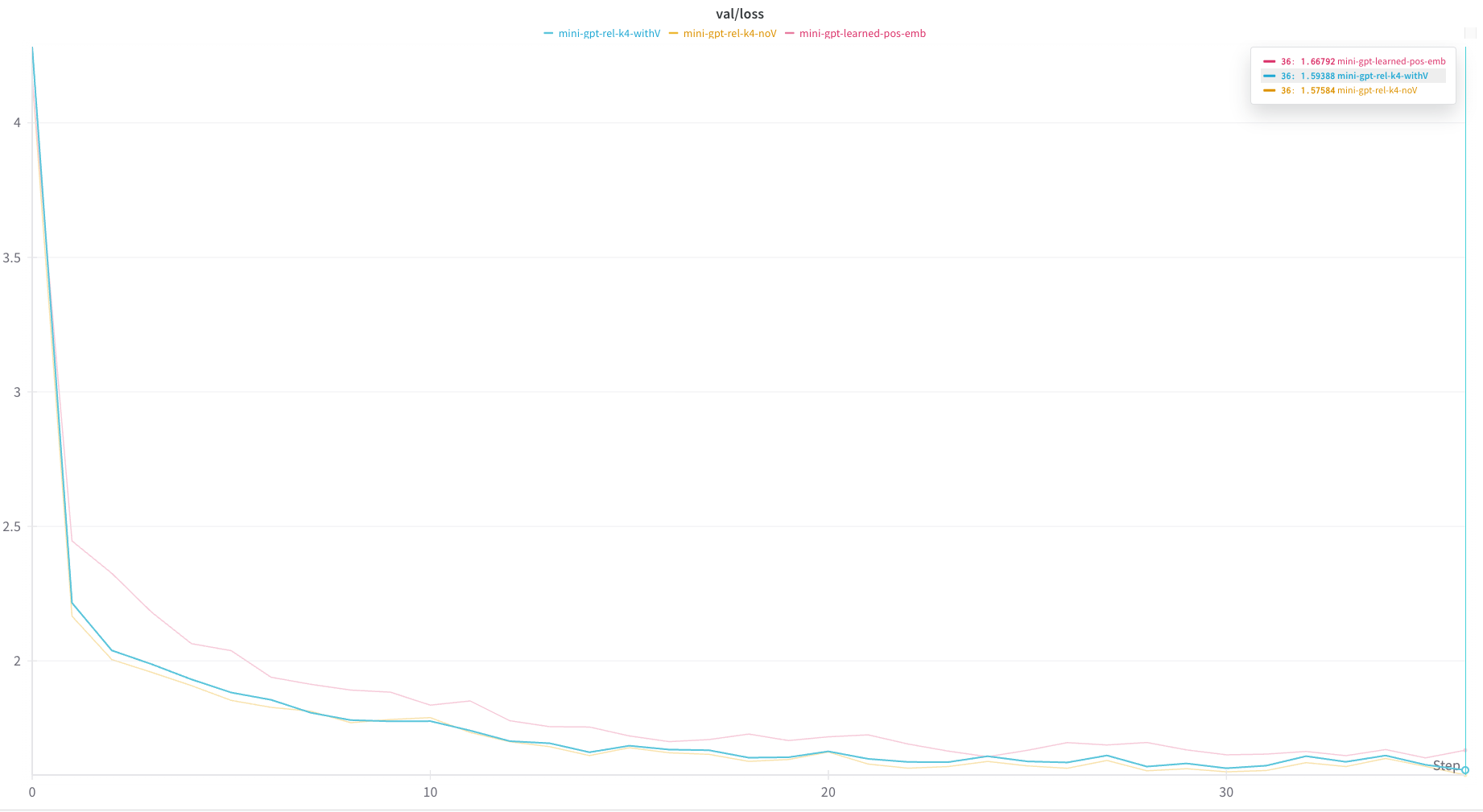
The relative position encodings out performed the learned absolute position encodings by a small amount, which is similar to the findings in the paper.
Further, I experimented with disabling the rV calculation and, and actually got slightly better results without rV.
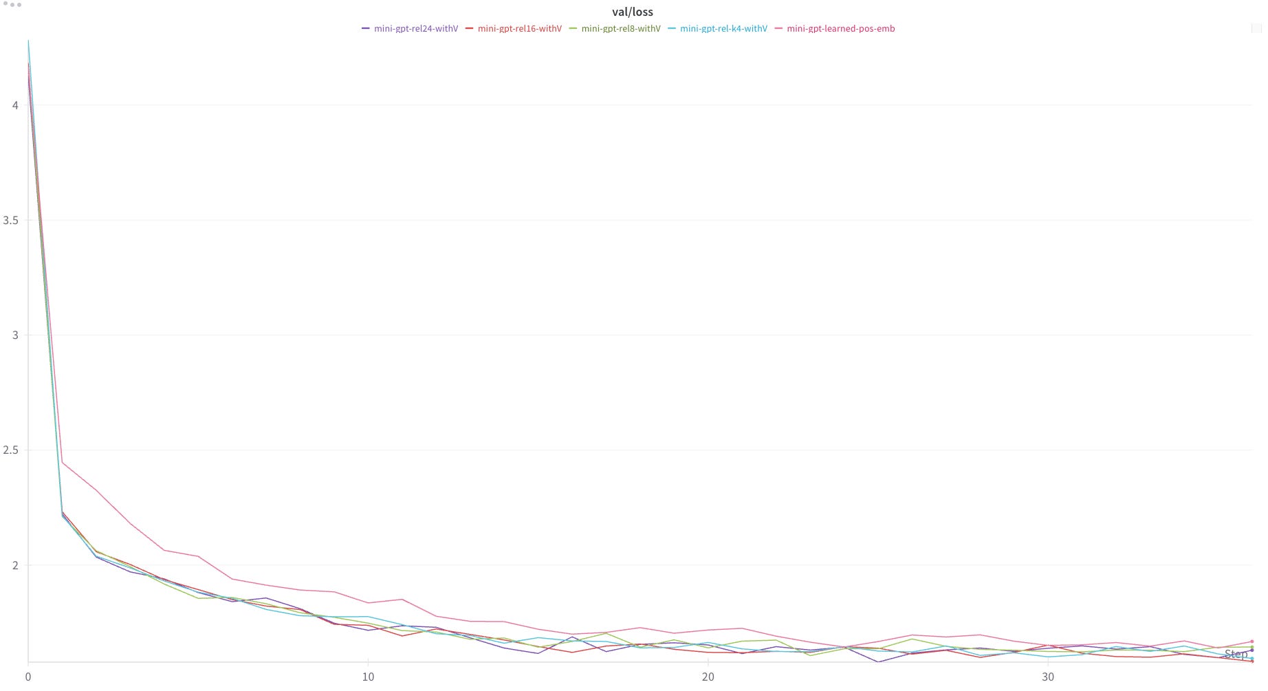
Finally, I also ran this calculation with other values of k (k=8, k=16, k=24).
Similar to the findings in the paper, I found that all values of k outperformed the learned absolute position embeddings, but larger values of k did not make a significant difference in overall performance.
Conclusion
Relative position embeddings improved upon learned absolute position embeddings, in terms of absolute performance on a validation dataset. In addition, since they do not depend on sequence input length, they do not place any limitations on the lengths of sequences that can be predicted using models with this embedding schema. This is a significant benefit of this encoding scheme — particularly in a world where context lengths are often tens if not hundreds of thousands of tokens long.
The performance improvement, as well as the ability to handle any input length, rest on the fact that this encoding scheme seems to capture the core reason a model would care about token position at all. Namely, it directly encodes the way token positions relate to each other.
Of course, this idea has been improved upon a number of times since its publication in 2018. The most important of these is Rotary Position Embeddings (RoPE), which combines the absolute sinusoidal positional embeddings with relative positional embeddings to great effect.
More on this next time.